Execution Plan is like a blueprint. SQL Server uses this to execute a DML query. As a DBA, understanding execution plans is like reading the X-ray of query performance. It exposes where SQL Server spent its time and resources, which indexes used or ignored, and area of performance bottlenecks.
In this article, you will go through how to analyze SQL Server execution plans, interpret key operators, and identify optimization opportunities.
Before proceeding further, you may wish to check my article about key concepts of execution plan.
- Understanding Execution Plan Part-1
- Understanding Execution Plan Part-2

Figure-1: Analyzing execution plan
Execution Plan
An execution plan is a step-by-step strategy that outlines how the execution engine will process the query, including how and when the indexes and tables will be accessed, the order of operations, and how data will be joined and filtered, foreign keys accessed and more. There two types of execution plan:
- Estimated plan - it represents the results coming from the query optimizer.
- Actual plan - it is estimated plan along with some runtime metrics.
How SQL Server Generates Execution Plan
Once a DML query is submitted to SQL Server, it goes through a series of steps. Each step does its own tasks and forwards the output to next step. Execution plan is generated at Optimizer step. Optimizer tries to find out the cheapest, not the best, cost-effective execution plan. Thus, it evaluates different permutations of indexes, statistics, constraints, and join strategies. This process could be time-consuming. So, it is divided the tasks into multiple sub-phases of optimization. Each sub-phase applies transformation rules to find a "cheapest" plan rather than a "best" one. If a plan’s estimated cost is acceptable after a phase, the optimizer stops immediately. Otherwise, it proceeds to the next phase. This balance between optimization time and plan quality. However, this can sometimes result in sub-optimal performance.
Reading an Execution Plan
You can read an execution plan either from right to left or even left to right. Usually,
- Reading from the left side, you will see the logical flow of data.
- Reading from the right side, you will see the physical flow of data.
Most of the cases, reading it from right side is more appropriate as it demonstrates how data is retrieving in the execution plan. However, sometimes the only way to understand what is happening in an execution plan is to read it in the logical processing order, left to right.
Characteristics of an Execution Plan
Paste below Query Snippet:-1 on AdventureWorks2022 database and generate the estimated execution plan by pressing Ctrl+L as shown in Figure-2.
SELECT
    p.BusinessEntityID
    ,p.FirstName
    ,p.LastName
    ,a.City
    ,p.EmailPromotion
    ,p.ModifiedDate
FROM Person.Person AS p
INNER JOIN Person.BusinessEntityAddress AS bea ON p.BusinessEntityID = bea.BusinessEntityID
INNER JOIN Person.Address AS a ON bea.AddressID = a.AddressID
WHERE p.LastName LIKE 'S%'
AND a.City IN ('Seattle', 'Dallas')
ORDER BY a.City

Query Snippet:-1
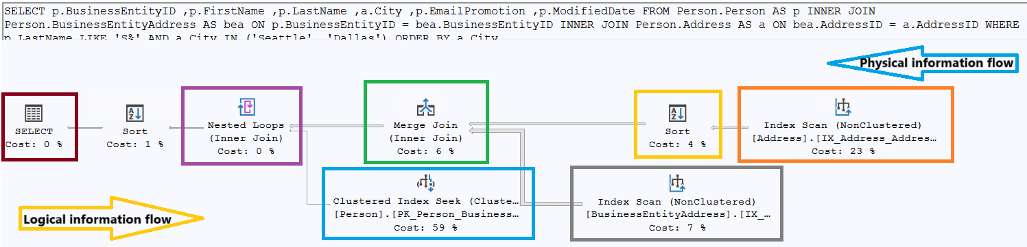
Figure-2: Execution Plan
There are some characteristics of execution plan:
- Under every operator, there is cost parameter which shows how much cost associated with this operator.
- This is relative to other operators and expressed as %.
- This is simply estimated cost unit assigned by the query optimizer.
- It indicates a mathematical construct of I/O and CPU usage.
- This is not the exact use of I/O and CPU.
- If a batch contains multiple queries, SQL Server displays an execution plan for each one in the order they are executed. Each plan shows its relative estimated cost. The total cost of all plans in the batch are 100%.
- Every icon is an operator and it has relative cost. The total cost of all operators are 100%.
- Sometimes, due to inaccurate statistics or bug of SQL Server, the total cost of all operators may not be 100%.
- If you read the execution plan from right to left (physical flow of data), then:
- 1st node(s) usually a data retrieval node.
- Data retrieval node is related to either table or index operation.
- Index operation will be either scan or seek. Like clustered index scan, clustered index seek, index scan, or index seek.
- The naming convention of a data retrieval operation is [Table Name].[Index Name].
- Arrow represents data flow between operators. Data flows from right to left.
- Thickness of arrow indicates number of row transferred.
- An operator displays both physical and logical operation types. If both operations are the same, then only the physical operation is shown. There are are also other information like row count, I/O cost, CPU cost, and so on.
- Physical operation - represent those actually used by the storage engine
- Logical operation - the optimizer uses this to build the estimated execution plan.
Analyzing an Execution Plan
When you analyze an execution plan, observe carefully below stuffs:
- Find out the warning (if any) which is represented by an exclamation point on one of the operators. Waring may arise due to various reasons. The most common issues are:
- A join without join criteria or an index or a table with missing statistics.
- Implicit datatype conversion. For example varchar to int.
- Cardinality estimate mismatch when actual vs. estimated row counts differ significantly.
- For a batch of statements, check the most costly estimated statement. You will see execution plan for each statement in the order they are executed. Each plan shows its relative estimated cost.
- In a single execution plan, each node displays its relative estimated cost with respect to total cost 100%. Pay attention on the nodes with the highest relative cost. For example in Figure-2, Clustered Index Seek part has the most cost 59%.
- Look for the thickness of the connecting arrows between nodes. The thicker the arrow the larger number of rows are transferred. Ask why so many data is transferred from the left of the arrow. May be:
- The estimated rows and the actual rows may differ due to out-of-date statistics.
- Index is not used.
- If there are thick arrows between most of the connecting nodes and then a thin arrow at the end, think of modifying the query or indexes to get the filtering done at origin.
- Search for any key lookup operator. Consider your indexes and try to use covering index. Check my previous article here.
- Examine hash join operations which is usually used for large data set. For small result sets, a nested loop join is preferable. Both join operations are fine. However, a nested loop works efficiently on small data set and a hash join on large set.
- Watch for sort operation which tells that the data was not retrieved in the correct sort order. It may not be an issue, but may be symptom of a missing or incorrect index. Sorting data using ORDER BY is not problematic. However, remember that sorting has negative impact on performance.
- Check for the table spool operation. It may be required for the query execution. This is an indication of sub-optimal query or a poor indexing. Consider this is a red flag as it puts extra load on CPU, memory, and TempDB.
- Be cautious about parallel query execution. A large query may get benefits by using multiple CPU cores, but it also increases CPU utilization and coordination overhead. Excessive parallelism can cause CXPACKET or CXCONSUMER waits which leads to contention between threads. Usually, it degrades performance for smaller queries due to synchronization and resource scheduling costs.
- Inspect for index scan and seek operations. When you need a few rows, seek operation is the best. For selecting all rows, scan is preferable. Check that optimizer is using the appropriate operator based on the purpose of your query.
- For retrieving data efficiently, optimizer selects the best index from the available indexes. If a desired index is not available, it uses the next best index and so on. For best performance, you should always ensure that the best index is used in a data retrieval operation.
- Investigate your join operations. There are four types of join. None of them are inherently good or bad. Sometimes, optimizer may pick inappropriate join types due to out-of-date statistics. So focus on the places where the optimizer pick the join type not aligned with the purpose of your query. Let's quickly evaluate all the join types:
- Hash Join - When there is no useful indexes, this join uses a hash table to match rows between two input sets namely build input and a probe input. It performs well on large, unsorted and non-indexed input datasets. However, it consumes more memory and CPU. This is less efficient for small datasets or when data is already sorted.
- Merge Join - A merge join requires both inputs to be sorted on the join key and then merge them in a single pass (means each input is scanned once in sorted order, not multiple times). It is very efficient for large and pre-sorted datasets. There is sorting overhead if no index exists or dataset is unsorted.
- Nested Loop Join - This join compares each row from one table (outer) with matching rows from another (inner). It works best when the outer input is small and the inner table is indexed but can perform poorly on large datasets without indexes.
- Adaptive Join - It dynamically chooses between hash and nested loop joins during query execution based on the actual row count. It improves performance when cardinality estimates are uncertain. There is minor runtime overhead for decision-making.
Some Stuffs Relevant to Execution Plan
There are some key stuffs which will help to troubleshoot or analyze an execution plan further.
Plan Cache
Once an execution plan is generated, SQL Server preserves it in memory for future use. So next time same query arrives, SQL Server does not repeat the costly plan generation process. Rather, it reuses the older one. Sometimes you may wish to check plan from plan cache. As SQL Server may old plan. Use below Query Snippet:-2 to retrieve plan from plan cache.
SELECT qp.query_plan, st.text
FROM sys.dm_exec_cached_plans cp
CROSS APPLY sys.dm_exec_query_plan(cp.plan_handle) qp
CROSS APPLY sys.dm_exec_sql_text(cp.plan_handle) st
WHERE st.text like 'SELECT%'

Query Snippet:-2
Plan Comparison
You can compare two plans and identify key differences between them. This will help you to optimize the query. First save your reference plan by right clicking on the plan and click on the "Save Execution Plan As..." option. Then open your target plan, right click and choose "Compare Showplan" and select your saved reference plan.
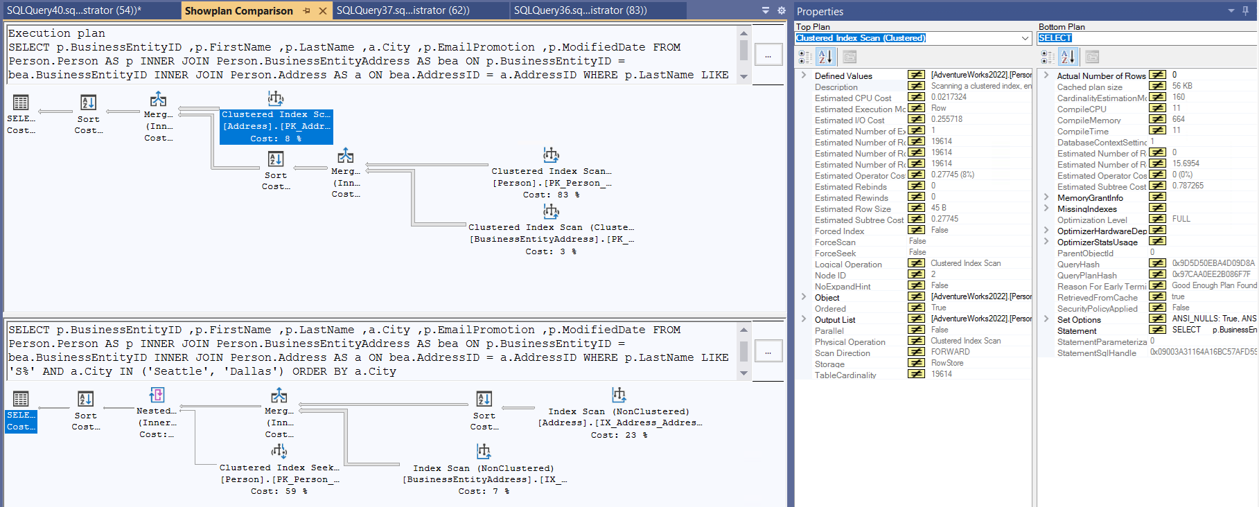
Figure-3: Plan comparison
Client Statistics
This is a great tool to capture execution metrics from the perspective of client machine (from where the query is executed) as shown in Figure-4. It records the time it takes to transfer data across the network from client machine. Not the time involved on the SQL Server machine. This is particularly helpful for troubleshooting a query. Even it shows data if you trial the query multiple times. To configure client statistics, from SSMS go to Query menu->Include Client Statistics menu item.
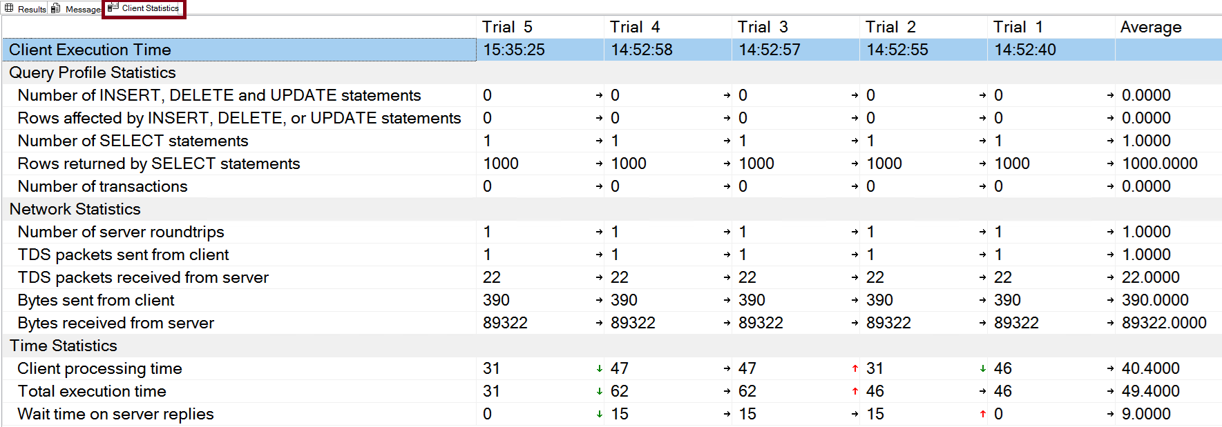
Figure-4: Plan comparison
Client statistics has some limitations:
- Collects limited set of data.
- Can not show how one execution is different from another.
- You could even run a completely different query, and its data would be mixed in with the others. This make the averages useless.
You can reset the client statistics by clicking Query menu->Reset Client Statistics menu item.
STATISTICS TIME and STATISTICS IO
STATISTICS TIME provides the time a query takes to execute which allows you to compare between different query versions to see which is faster and more efficient.
- CPU time - The total time the query spent actively running on the CPU. This is a good metric for comparing performance, as it is not affected by other processes.
- Elapsed time - The total time from when the query started to when it finished. This can be longer than CPU time if the query is waiting for other processes or resources.
STATISTICS IO helps to measure the amount of physical and logical IO activity generated by a query. So, you can identify which parts of a query are doing excessive disk activity. This is crucial for performance tuning.
- Physical IO is related to accessing data pages on disk
- Logical IO is related to accessing data pages in memory (data cache).
You can enable both STATISTICS TIME and STATISTICS IO using below Query Snippet:-3.
SET STATISTICS IO ON;
GO
SET STATISTICS TIME ON;
GO

// Your Queries go here

GO
SET STATISTICS TIME OFF;
GO
SET STATISTICS TIME OFF;
GO

-------- Or you can use them together --------
SET STATISTICS IO, TIME ON;
GO

// Your Queries go here

SET STATISTICS IO, TIME OFF;
GO

Query Snippet:-3
Final Words
Analyzing execution plans is one of the most powerful skills for a DBA. By carefully examining operators, join types, costs, and potential warnings, you can uncover performance bottlenecks that remain hidden at the query level. That will help you to tune queries, design better indexes, and ensure the optimizer works in your favor. In short, mastering execution plan analysis bridges the gap between query design and real-world performance.
References
Going Further
If SQL Server is your thing and you enjoy learning real-world tips, tricks, and performance hacks—you are going to love my training sessions too!
Need results fast? I am also available for 1-on-1 consultancy to help you troubleshoot and fix your database performance issues.
Let’s make your SQL Server to take your business Challenge!
For any queries, mail to mamehedi.hasan[at]gmail.com.